Implementation#
This section will introduce the idea of all the spatial analysis methods and algorithms use in spatialtis.
Hopefully the following explanation can help you understand it as easily as possible.
Determine cell shape#
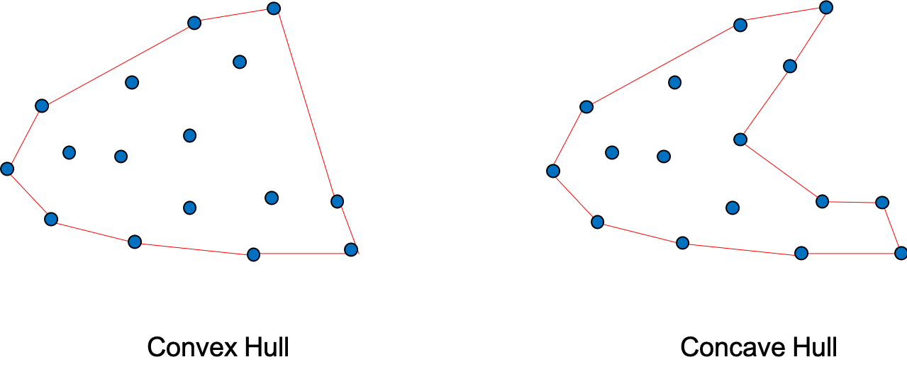
There are two way to determine the shape of a cell, “convex hull” or “concave hull”. The “concave hull” is slower and need an extra parameter, an alpha value. This will influence the cell_shape but no other geometry information.
Cell co-occurrence#
The occurrence or absence of a cell type in a ROI (Region of interest) is determined by a threshold value, the default is mean cut. The cell type is determined as occurrence if it’s counts exceed 50 otherwise it’s absence. Afterwards, if two types of cell are both determine as occurrence, one-way \(\chi^2\) test are conducted to determine the significance, if one or both are absence would be determined as non co-occurrence.
Find cell neighbors#
Depends on the resolution of different spatial single-cell technology, some resolved single cell as point, another with subcellular resolution can resolve single cell in 2D-shape. For each ROI, every cell will be stored in a spatial index tree structure allowing for fast neighbor search.
For point data, KD-tree is used and constructed using kiddo.
For 2D-shape data, R*-tree is used and constructed using rstar.
Profiling of cell-cell interaction#
To profile the interaction between cells, spatialtis used permutation test. First purposed in histocat.
Let’s simplify the situation here, consider only the interaction between cell type A and B. We can draw a distribution from the real dataset of the number of Cell B at the neighborhood of Cell A. After that, we can randomize the dataset, randomly reassign cell type to different cell while keep the number of each cell type unchanged. Therefore we can draw another distribution. This randomization process can perform multiple times (usually 1000 times) to draw a null distribution.
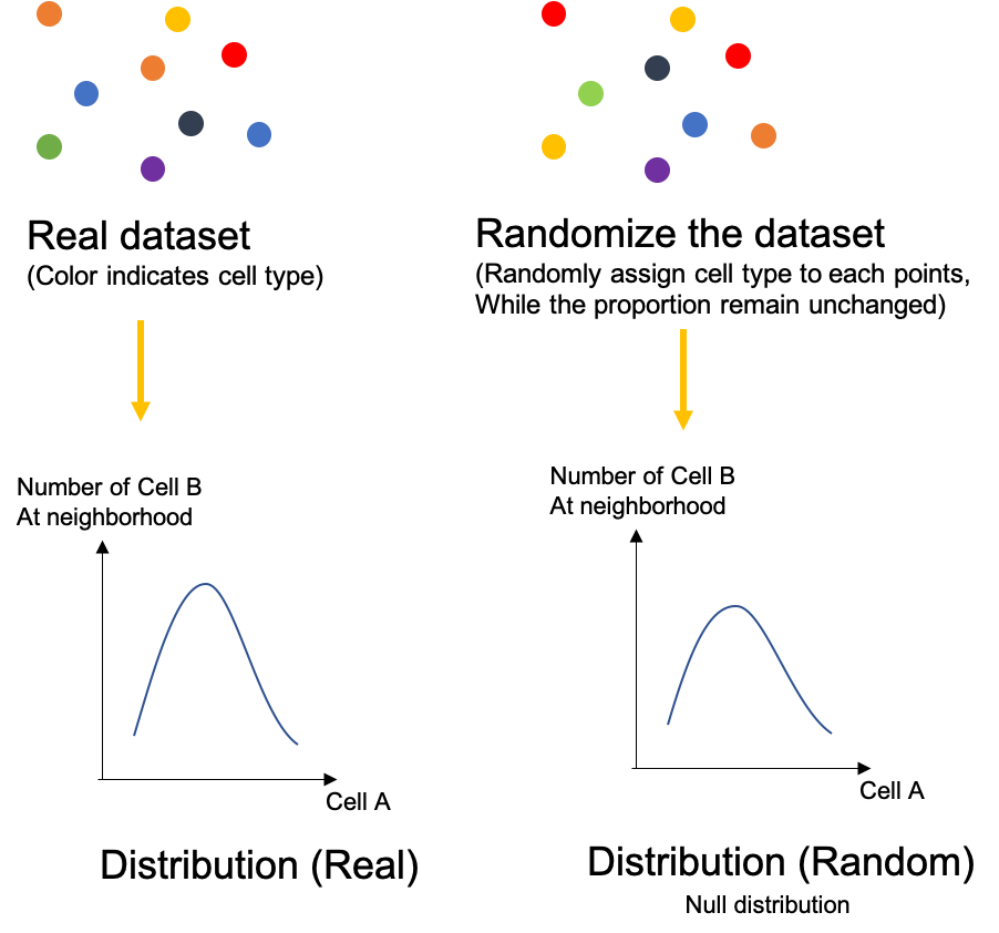
Now let’s compare the difference between two distributions. If the distribution from the real has less difference to the distribution from the random dataset, it means the real distribution might just be random whereas the relationship between Cell A and B is likely to be random. But if there is a significant differences, the relationship between Cell A and B could likely to be association (If many Cell B around Cell A) or avoidance (If few Cell B around Cell A).
In neighborhood analysis, a pseudo-p value is calculated as follow:
Or using z-score:
Profiling of markers enrichment#
User defines the positive / negative of a marker in a cell, same bootstrap method is conducted as above. A z-score is calculated for each combination of markers.
Spatial distribution#
There are three point distribution patterns in general, random, regular and cluster. Random means the point pattern follows the poisson process, the regular means evenly distributed and cluster means the points tend to aggregate. (Cells are represented by their centroid)

To determine the cell distribution patterns in each ROI, spatialtis provided three methods.
Index of Dispersion (ID)
Morisita’s index of dispersion (MID)
Clark and Evans aggregation index (CE)
Random |
Regular |
Clumped |
|
|---|---|---|---|
Index of dispersion: ID |
ID = 1 |
ID < 1 |
ID > 1 |
Morisita’s index of dispersion: I |
I = 1 |
I < 1 |
I > 1 |
Clark and Evans aggregation index: R |
R = 1 |
R > 1 |
R < 1 |
Index of dispersion#
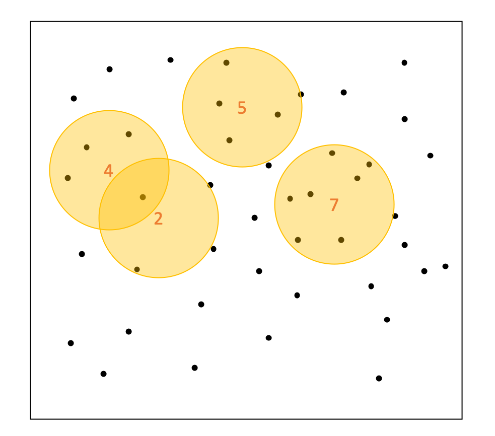
Sampling process, the orange circle is the sampling windows, the number is the count of points#
First we store all the point in a ROI in KD tree. A random sample window with diameter r is generated, the count of points in this window is x, a number of counts are generated after sampling many times. The null hypothesis is that the points are randomly distributed. \(s^2\) is the variance of all samples, \(\overline{x}\) is the average of all samples. Index of dispersion is calculated as follow:
Morisita’s index of dispersion#
This is a quadratic statistic method, user need to define how to rasterize the ROI.
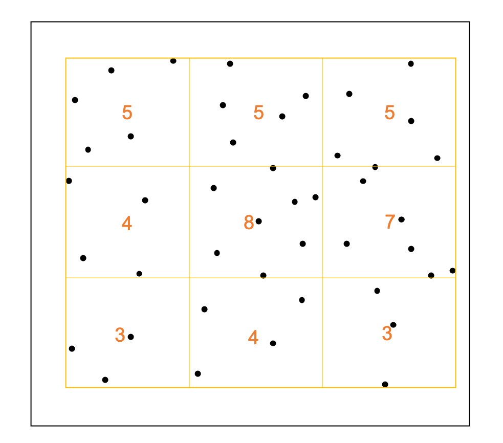
In this example, the ROI is divided into \(3\times3\) grids, the number is the count of points#
Morisita’s index of dispersion is calculated as follow:
\(\sum x\) sum of the quadrat counts \(\sum x = x_1+x_2+x_3+...\)
\(\sum x^2\) sum of quadrat counts squared \(\sum x = x_1^2+x_2^2+x_3^2+...\)
\(\chi^2 = I_d(\sum x - 1)+n-\sum x\) (\(df = n-1\))
Clark and Evans aggregation index#
This method evaluate the distribution pattern base on distance between points. The points are stored in KD tree at the first place.
Index of aggregation is calculated as follow:
\(\rho\) density of individuals: \(\rho = \frac{n}{\text{area}}\)
\(n\) number of individuals
Spatial heterogeneity#
In spatialtis, three entropy methods have been implemented to quantify the heterogeneity in a ROI. Shannon entropy doesn’t consider the spatial information. The Leibovici entropy and Altieri entropy consider spatial factor to evaluate entropy in a system. See spatialentropy.
Shannon entropy#
To compare the difference within a group (eg. different samples from same tumor), Kullback–Leibler divergences for each sample within the group are computed, smaller value indicates less difference within group.
Leibovici entropy#
Leibovici entropy is based on the shannon entropy. A new variable \(Z\) is introduced.
\(Z\) is defined as co-occurrences across the space. For example, we have \(I\) types of cells. The combination of any two type of cells is \((x_i, x_{i'})\), the number of all combinations is denoted as \(R\).
If order is preserved, \(R = P_I^2 = I^2\);
If the combinations are unordered, \(R = C_I^2= (I^2+I)/2\).
At a user defined distance \(d\), only co-occurrences with the distance \(d\) will take into consideration.
The Leibovici entropy is defined as:
Altieri entropy#
Altieri entropy introduce another new vairable \(W\). \(W_k\) represents a series of sample window, i.e. \([0,2][2,4][4,10],[10,...]\) while \(k=1,...,K\).
The purpose of this entropy is to decompose the spatial entropy into Spatial mutual information \(MI(Z,W)\) and Spatial residual entropy \(H(Z)_W\).
The Altieri entropy is defined as:
The Spatial residue entropy is defined as:
The Spatial mutual information is defined as:
Hotspot detection#
Hotspot detection is used to find the cells that form clumps. Here we use Getis–Ord hotspot analysis. First we rasterize the ROI into grids, for each small square, we will compare it to its neighbor cells. User can define the level of neighbors to search.
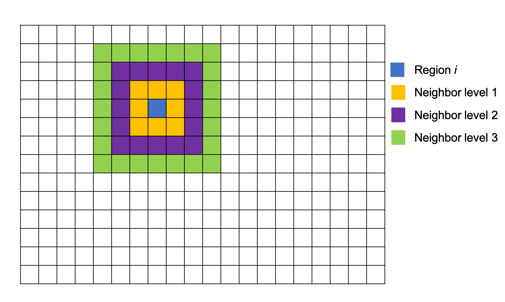
z score for a region \(i\):
\(n\) total number of grid regions
\(C_j\) Cell count for region j
\(\overline{C}\) mean of cell count in all region
Communities detection#
This is used to find communities in a ROI. The neighbors relationships are convert to graph, each cell is a node, two nodes are connected if they are neighbors, edge weight is represented by distance. Using leidenalg algorithm, we can detect the communities within a ROI.
Spatial Co-expression#
For all pair of neighbor cells, to compute the correlation between two markers \(A\) and \(B\). Two vector can be constructed, \({\{A_1, A_2, ..., A_x\}}\) \({\{B_1, B_2, ..., B_x\}}\). \(A_1\) is the expression of marker \(A\) in \(Cell N\), \(B_1\) is the expression of marker \(B\) in \(Cell M\). \(Cell N\) and \(Cell M\) is a pair of neighbor. In spatialtis, pearson or spearman correlation can be computed.
Neighbor dependent markers#
This method tells you the dependency and correlation between markers and its neighbor cell/markers. The dependency is calculated by building a gradiant boosting tree (in here LightGBM) to determine the feature importance. And the the spearman correlation is calculated.