IMC diabetes dataset, 1.8 Million cells#

This example shows some of the analysis and visualizations in SpatialTis.

It should give you a general idea on how to use it.

[1]:

%config InlineBackend.figure_format = 'retina'
import anndata as ad
import spatialtis as st
import spatialtis.plotting as sp
from spatialtis import Config

[2]:

data = ad.read_h5ad("../data/IMC-diabetes.h5ad")
data.obs.head(5)

[2]:

	area	eccentricity	centroid	image	case	slide	part	group	stage	cell_cat	cell_type	n_genes
0	12	0.837664	(52.5, 0.6666666666666666)	A01	6362	A	Tail	1	Onset	exocrine	acinar	30
1	19	0.902864	(128.0, 0.894736842105263)	A01	6362	A	Tail	1	Onset	exocrine	acinar	36
2	7	0.882300	(135.28571428571428, 0.42857142857142855)	A01	6362	A	Tail	1	Onset	exocrine	acinar	30
3	19	0.784367	(449.5263157894737, 1.1578947368421053)	A01	6362	A	Tail	1	Onset	exocrine	acinar	33
4	30	0.930895	(458.3666666666666, 1.1)	A01	6362	A	Tail	1	Onset	exocrine	acinar	38

[3]:

data

[3]:

AnnData object with n_obs × n_vars = 1776974 × 38
    obs: 'area', 'eccentricity', 'islet_id', 'centroid', 'image', 'case', 'slide', 'part', 'group', 'stage', 'cell_cat', 'cell_type', 'n_genes'
    var: 'markers', 'n_cells', 'highly_variable', 'means', 'dispersions', 'dispersions_norm'
    uns: 'hvg'

[4]:

st.wkt_points(data, 'centroid')

[5]:

Config.exp_obs = ['stage', 'part', 'case', 'image']
Config.centroid_key = 'centroid'
Config.cell_type_key = 'cell_type'
Config.marker_key = 'markers'
Config.progress_bar = False

Check the configuration to make sure things are correct

[6]:

Config.view()

                      Current configurations of SpatialTis                      
┏━━━━━━━━━━━━━━━━━━━━━━━━━┳━━━━━━━━━━━━━━━┳━━━━━━━━━━━━━━━━━━━━━━━━━━━━━━━━━━━━┓
┃ Options                 ┃ Attributes    ┃ Value                              ┃
┡━━━━━━━━━━━━━━━━━━━━━━━━━╇━━━━━━━━━━━━━━━╇━━━━━━━━━━━━━━━━━━━━━━━━━━━━━━━━━━━━┩
│ Multiprocessing         │ mp            │ True                               │
│ Verbose                 │ verbose       │ True                               │
│ Progress bar            │ progress_bar  │ False                              │
│ Auto save               │ auto_save     │ False                              │
│ Experiment observations │ exp_obs       │ ['stage', 'part', 'case', 'image'] │
│ ROI key                 │ roi_key       │ image                              │
│ Cell type key           │ cell_type_key │ cell_type                          │
│ Marker key              │ marker_key    │ markers                            │
│ Centroid key            │ centroid_key  │ centroid                           │
│ Shape key               │ shape_key     │                                    │
└─────────────────────────┴───────────────┴────────────────────────────────────┘

Save the config to the data

[7]:

Config.dumps(data)

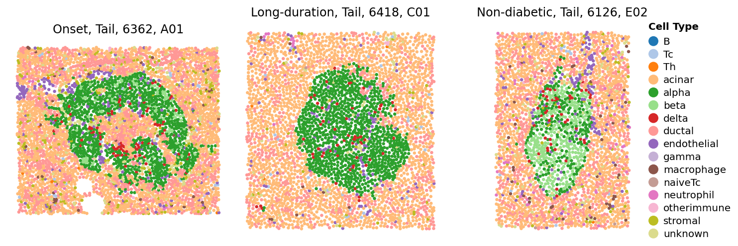
Let’s look at what those ROI looks like

[8]:

sp.cell_map(data, ['E02', 'A01', 'C01'])

[8]:

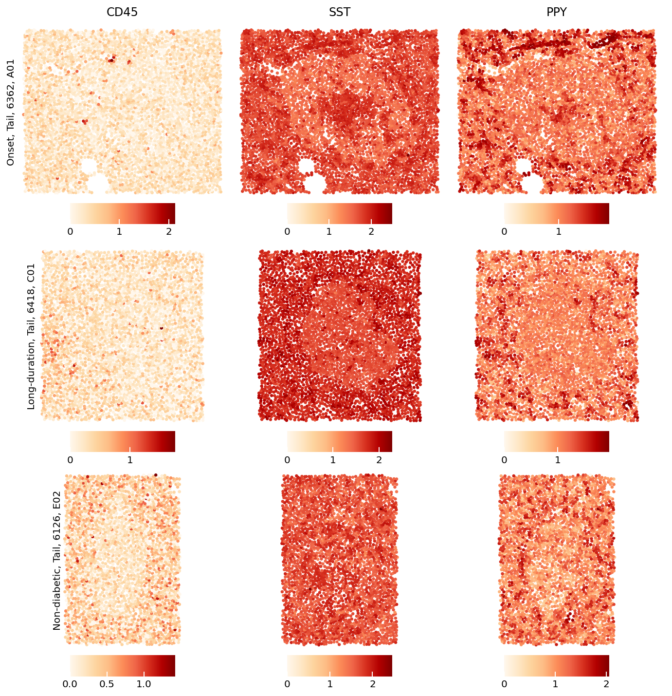
[9]:

sp.expression_map(data,
                  rois=['E02', 'A01', 'C01'],
                  markers=['CD45', 'SST', 'PPY'])

[9]:

[10]:

st.cell_components(data)

⏳ Cell components

📦 Added to AnnData, uns: 'cell_components'

⏱ 3s510ms

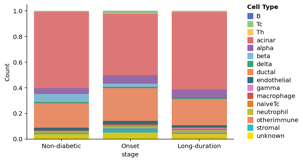
[11]:

sp.cell_components(data,
                   groupby='stage',
                   percentage=True,
                   order=['Non-diabetic', 'Onset', 'Long-duration'])

[11]:

<AxesSubplot:xlabel='stage', ylabel='Count'>

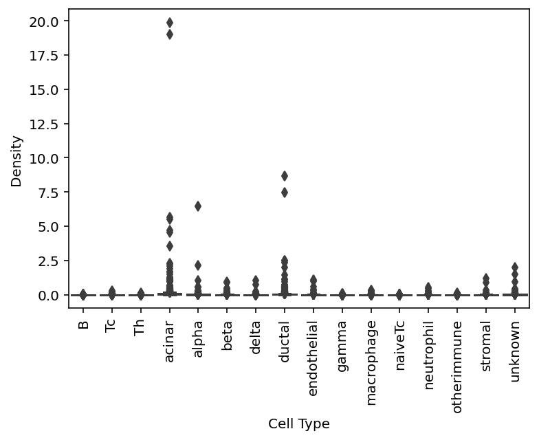
[12]:

st.cell_density(data)

⏳ Cell density

📦 Added to AnnData, uns: 'cell_density'

⏱ 9s413ms

[13]:

sp.cell_density(data)

[13]:

<AxesSubplot:xlabel='Cell Type', ylabel='Density'>

[14]:

st.cell_co_occurrence(data)

⏳ Cell co-occurrence

📦 Added to AnnData, uns: 'cell_co_occurrence'

⏱ 3s455ms

[15]:

sp.cell_co_occurrence(data)

[15]:

<milkviz._dot_matrix.DotHeatmap at 0x25e129cbdf0>

[16]:

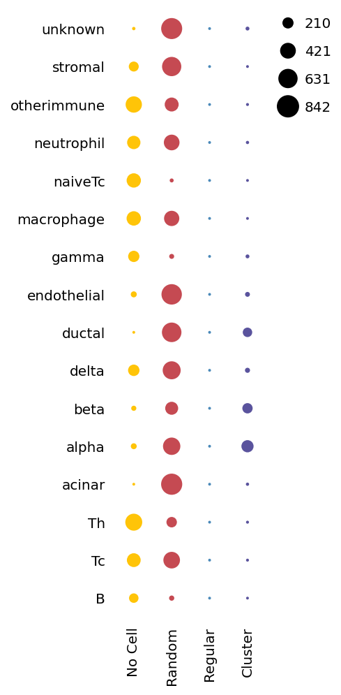
st.cell_dispersion(data)

⏳ Cell dispersion

🛠 Method: Index of dispersion

📦 Added to AnnData, uns: 'cell_dispersion'

⏱ 9s716ms

[17]:

sp.cell_dispersion(data)

[17]:

<milkviz._dot_matrix.DotHeatmap at 0x25e8b5ce250>

[18]:

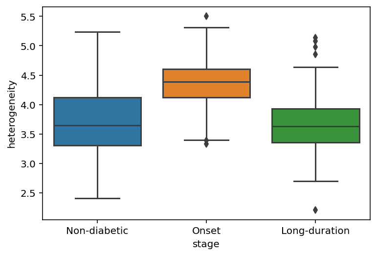
st.spatial_heterogeneity(data)

⏳ Spatial heterogeneity

🛠 Method: Leibovici entropy

📦 Added to AnnData, uns: 'heterogeneity'

⏱ 7s587ms

[19]:

sp.spatial_heterogeneity(data, order=['Non-diabetic', 'Onset', 'Long-duration'])

[19]:

<AxesSubplot:xlabel='stage', ylabel='heterogeneity'>

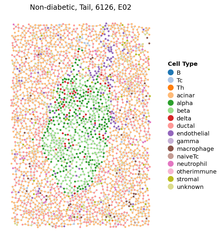
One of the most essetial steps in analyzing spatial omics data is to embedding it into a spatial network.

[20]:

st.find_neighbors(data, r=12)

⏳ Find neighbors

🛠 Method: kdtree

📦 Added to AnnData, obsm: 'cell_neighbors'

📦 Added to AnnData, obs: 'cell_neighbors_count'

⏱ 10s976ms

[21]:

sp.cell_map(data, ['E02'], show_neighbors=True, figsize=(6, 7))

[21]:

[22]:

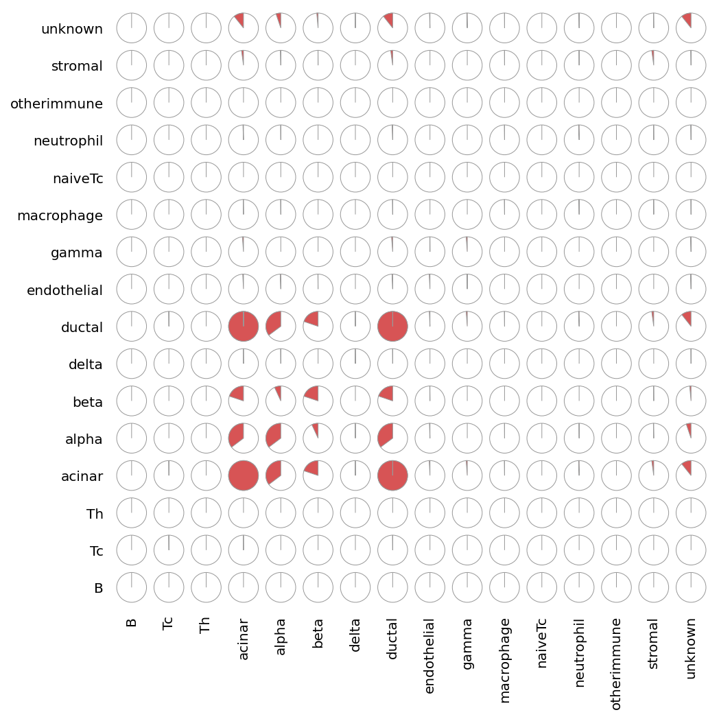
st.cell_interaction(data)

⏳ Cell interaction

🛠 Method: pseudo p-value

📦 Added to AnnData, uns: 'cell_interaction'

⏱ 1m56s

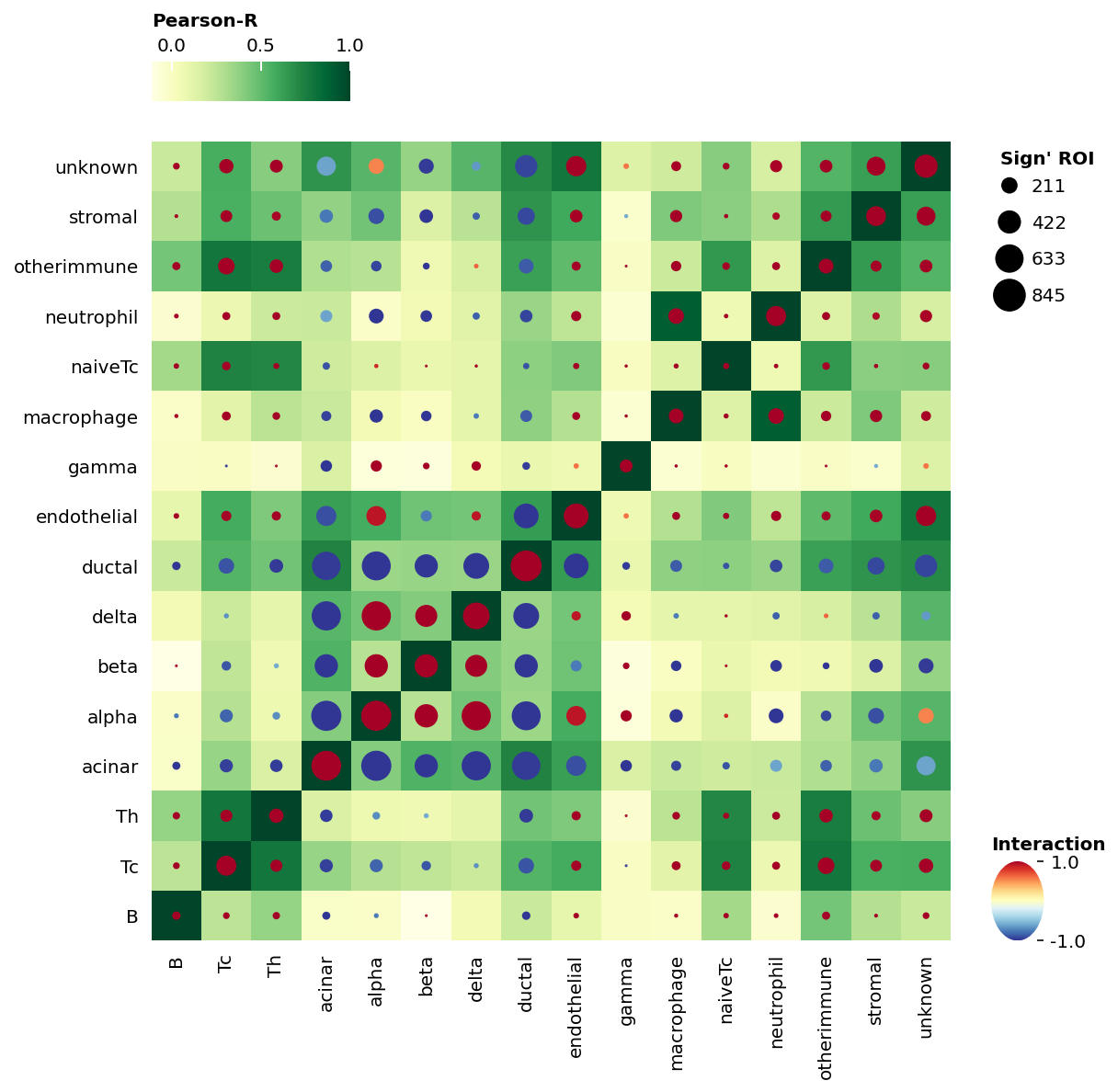
[23]:

sp.cell_interaction(data)

[23]:

<milkviz._dot_matrix.DotHeatmap at 0x25dd0175250>

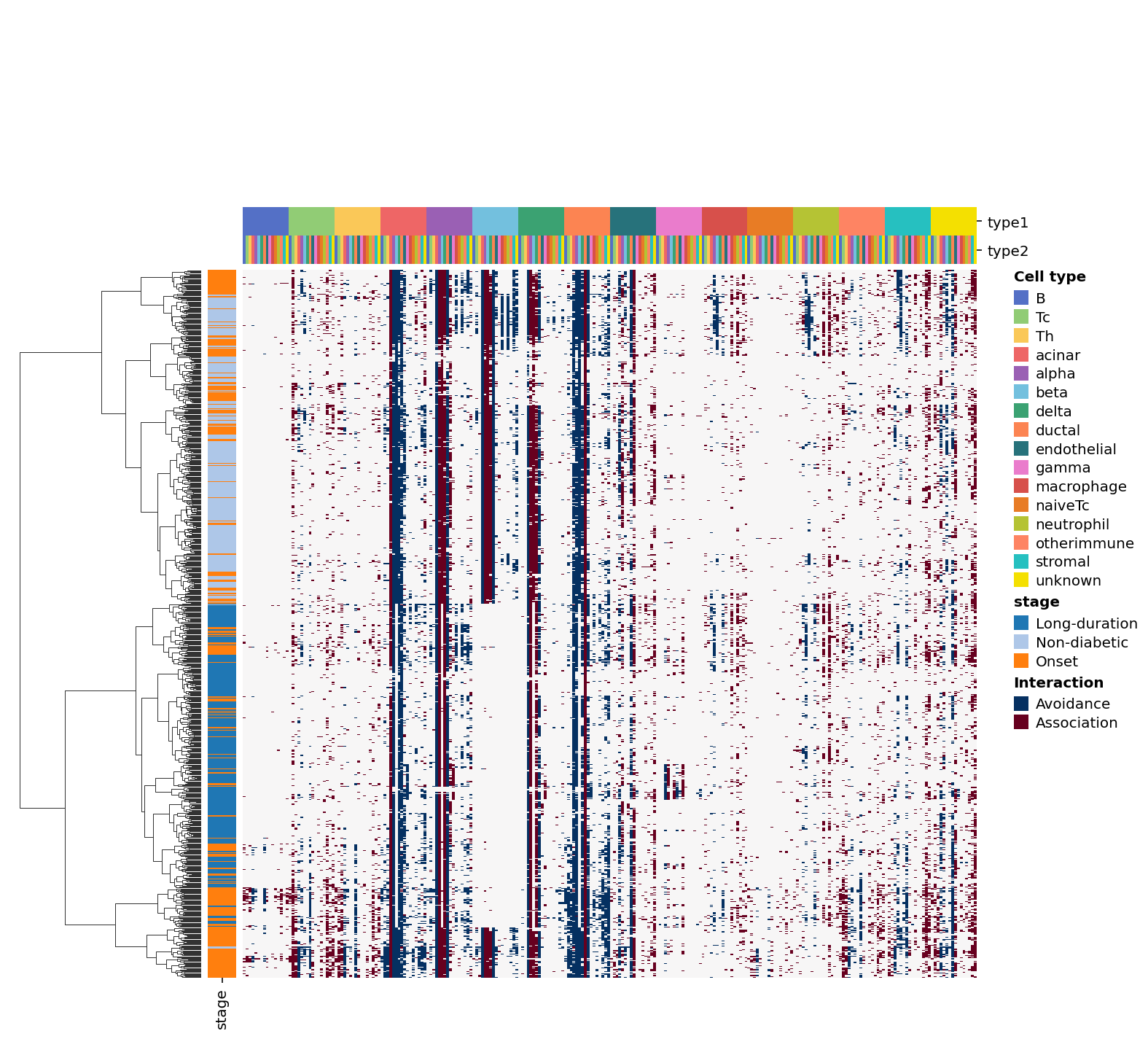
Or you can visualiza it in heatmap

[24]:

sp.cell_interaction(data, use="heatmap", groupby="stage")

[24]:

<seaborn.matrix.ClusterGrid at 0x25e449953d0>

[25]:

st.NCD_marker(data)

⏳ NCD Markers

📦 Added to AnnData, uns: 'ncd_marker'

⏱ 3m18s

[26]:

r = st.get_result(data, 'ncd_marker')
r.sort_values('log2_FC', ascending=False)

[26]:

	cell_type	marker	neighbor_type	dependency	log2_FC	pval
39	delta	CDH	gamma	0.914396	2.484879	3.493616e-279
34	beta	CDH	gamma	0.860546	2.417639	5.402380e-112
81	unknown	CDH	gamma	0.730400	2.405135	1.074318e-214
56	endothelial	CDH	gamma	0.542463	2.367553	5.895981e-90
75	stromal	CDH	gamma	0.528550	2.337943	2.023402e-33
...	...	...	...	...	...	...
31	alpha	cPARP1	beta	0.675172	-0.061171	0.000000e+00
44	delta	SST	beta	0.705842	-0.067218	0.000000e+00
19	alpha	CA9	beta	0.673017	-0.109999	0.000000e+00
37	delta	CA9	beta	0.653708	-0.142080	0.000000e+00
46	delta	cCASP3	beta	0.516018	-0.164905	6.121436e-302

87 rows × 6 columns

[ ]: